¶ Weights
¶ Tutorial 4 of Implementing Flappy Bird game to understand mathematical fundamentals behind neural networks
¶ Introduction to weights
In tutorial 2, we briefly described the structure of a fully-connected neural network. It was mentioned that the layers are fully connected and that every connection has a specific number; a weight. But what are weights, and why are they useful?
A weight is a number that represents the importance of the specific connection. Higher numbers will influence the output more than lower numbers. In the examples below, we have a simple network of two input nodes, and , and one output node . The connection between nodes and has a weight of , and the weight of differs in the examples.
We take the first example as a starting point. In this example, input node has more impact on the output value of node than input node since the weight of is higher.
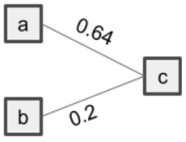
The weight of is near zero. Take a moment to think for yourself what will happen with the output of when increasing node and check the answer below.
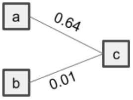
Solution
Weights near-zero means changing this input will not change the output. has a weight of in the example, which is near zero. Changing , so also increasing , barely affects the output of .
The weight of has a negative weight. What will happen with the output of when increasing node ?
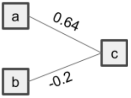
Solution
has a negative weight in the example. Negative weights mean increasing this input will decrease the output. So when increasing , the output of will decrease.
¶ Calculating node values
In a neural network, the weights of the first layer will be randomly generated. Every node in the next layer is calculated based on the weights from the previous layer. To explain how this calculation is performed, a network of two input nodes and three hidden nodes is demonstrated below. The values of the input nodes and the weights are randomly picked. With these values, we want to calculate the values of the three hidden nodes.
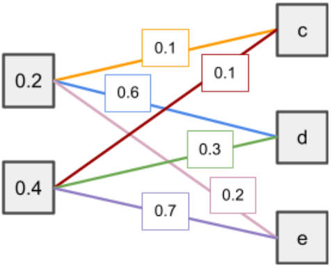
As explained in the previous tutorial, the principle of matrices can be used to calculate the values of the nodes. The first matrix of the input nodes can be written as a matrix of one column by two rows:
Also, the weight values can be written down in a matrix. In the example, we have in total six weights connecting two input nodes with three hidden nodes. The number of input nodes is equal to the number of columns in the matrix. Equivalent, the number of ‘output’ nodes, in this case, hidden nodes, equals the number of rows in the matrix. Transforming the weights into a matrix will result in the following:
Finally, the values of the three hidden nodes can be calculated by multiplying those two matrices according to matrix multiplication rule as explained in the previous tutorial:
The final matrix shows hidden node will get a value of , of , and is equal to .
¶ Applying weights in the Flappy Bird game
The python package we use during the Flappy Bird game for handling matrices is called NumPy. The main data structure in NumPy is an array. This type of structure is used to store a collection of elements of the same data type. In the matrices above we used floats[1], which will be the data type in our Flappy Bird game. Like matrices, an array can consist of rows and columns. Each row will be written as a list within the array. The number of elements in a row correspond with the number of columns.
NumPy has built-in functions to perform calculations with matrices. The NumPy function of matrix multiplication is named np.dot. Let us write the above matrices of the input values and weight values in an array and calculate the multiplication using NumPy.
import numpy as np

# Define the input values in a matrix
input_matrix = [
    [0.2],
    [0.4]
    ]

# Define the weights in a matrix
weights_matrix = [
    [0.1, 0.1],
    [0.6, 0.3],
    [0.2, 0.7]
    ]

# Perform matrix multiplication
np.dot(weights_matrix, input_matrix)
The output of the final code line prints array([[0.06], [0.24], [0.32]]). Indeed, these are the hidden nodes values as we calculated before.
¶ Activation functions
So far, we have used matrix transformation on the input. However, these calculations are like a simple linear model. To allow the neural network to learn powerful operations, it is necessary to add non-linearities into the network. We can do this by using so called activation functions.
Activation functions are inspired by the action potential in neuroscience, hence the name neural network. If the electrical potential in a neuron exceeds a value, the neuron undergoes a chain reaction which results in 'activating' and transmitting a signal to neighboring neurons. The same holds on in ‘pushing’ values of the neural network forward. We want that important values, higher values, have more influence and will be ‘activated’. An activation function will output a small value for small inputs, and a larger value if its inputs exceed a threshold.
There are several different activation functions, each having its own function. The one we will use is a well-known one, which is called logistic sigmoid. More information about (non-linear) activation functions and why to use them is explained here. The function of sigmoid is defined as:
Given this function, we see that every input value will be transformed to a value between 0 and 1. We can illustrate this better by showing the graph of the sigmoid function.
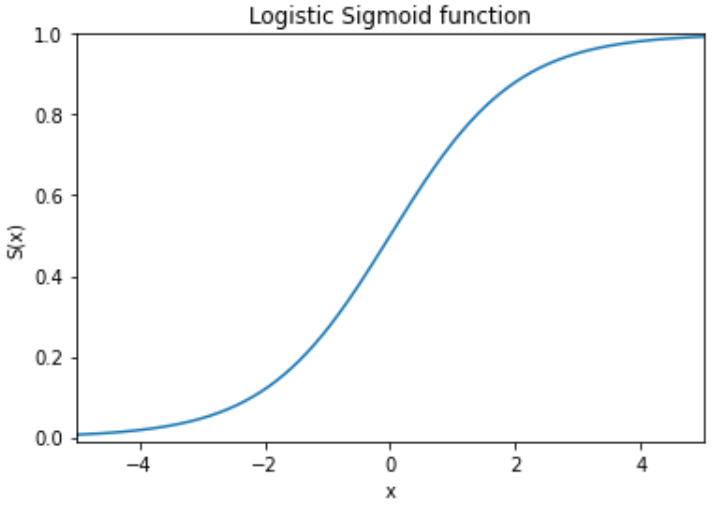
To make the neural network as powerful as possible, activation functions are applied on every calculated output value. We consider every value obtained after performing a calculation as an output value. So, transforming input values to hidden node values using weights by applying matrix multiplication, as we did above, gives output values. Let us apply an activation function on the calculated values of , and .
The Python SciPy package has a built-in function of logistic sigmoid. This function scipy.special.expit(x) transforms every value of a NumPy array and gives the same shaped array with sigmoid output values. To transform the values of , and , we can simply write the following code:
import numpy as np
import scipy.special

# Define the input array
hidden_inputs = np.array([[0.06], [0.24], [0.32]])

# Apply the sigmoid function on the input values
scipy.special.expit(hidden_inputs)
The output of the final code is array([[0.5149955 ], [0.55971365], [0.57932425]]). As expected by looking at the sigmoid graph above, all values will be around . In this case, there is no node that has a huge influence in comparison with the others.
¶ Final output value
In this tutorial, we have learned to transform input values into output values by first performing matrix multiplication with weight values, and subsequently applying an activation function. In the above example we have applied these steps to values of the input layer to go to hidden layer output values. The same principle can be applied by calculating the values of the output layer. In the case of the Flappy Bird game, we will get one final output value. The activation function on the output layer determines if the bird will flap (if the output value is equal or higher than ) or is doing nothing.
¶ Summary
In this tutorial, you have learned what weights are and how they fulfill a crucial role in neural networks. Moreover, you have also seen that an activation function is required to tell the neural network what to do. To make the neural network work, we use the Logistic Sigmoid function as an activation function. Finally, you have also seen how this activation function works in Python.
In the previous tutorials, you have learned the building blocks of neural networks and the tools to implement it. Therefore, we will get the AI working in the next tutorial and see if it can beat the game!
See the Python introduction Wiki for an recap of python syntaxes ↩︎