¶ Gradient descent
¶ Tutorial 7 of Implementing Flappy Bird game to understand mathematical fundamentals behind neural networks
¶ Introduction
In the previous tutorial, we have seen the importance of optimization, and we have seen how our current network optimizes the flappy bird. This tutorial will dive a little deeper into optimization, and particularly Gradient Descent. However, this tutorial will not include any code to improve the AI.
¶ Setting the derivative to 0
In high school mathematics, you have learned that you can find the maximum or minimum of a function by calculating the function's derivative and setting this to 0.
Minimize (or: find the minimum of) .
gives
Substituting in the formula for gives .
So the minimum is attained at with value .
¶ Approximating the maximum or minimum
Sadly enough, it is not always possible to simply compute the derivative and setting this to 0. Imagine that if you have a function that contains more than two variables, it gets harder and harder to differentiate, let alone computing extrema. Therefore, we need a way to get as close as possible to the maximum or minimum of our function. Gradient descent is such a method, but in order to use it, we will first need to learn two new concepts, namely the gradient and Steepest Descent.
¶ The gradient of a function
The gradient of a function is denoted with . So we denote the gradient of the function as or simply . For a one-variable function, the gradient is simply the derivative of that function.
Calculate of .
so .
The gradient gets more interesting for multivariable functions. We can compute the gradient for multivariable functions by taking a partial derivative of the function with respect to each variable.
Try computing the derivative of .
This was a trick question! We cannot compute 'the derivative' because we need to know if we want to compute the derivative with respect to or with respect to . The derivative of with respect to is denoted by and the derivative of with respect to is denoted by .
In this example, and .
The gradient of a two-variable function is given by
, so the gradient is a vector!
The gradient of a three-variable function is given by
and so on.
¶ Exercises on computing the gradient
Now that we have seen what the gradient of a function is, let us try some exercises.
Compute the gradient of .
and , so
Remember; when differentiating a function with respect to a certain variable, the other variables behave as constants! That is why the derivative of with respect to equals —the rest of the terms act as constants; hence their derivative equals 0.
Compute the gradient of .
and
So
¶ Gradient descent method for optimizing functions
We can use the gradient to approximate the minimum[1] of a function. The gradient of a function at a certain point gives us the graph's direction in that point. For simplicity, consider the case where we only have an and variable, and let us take the function:
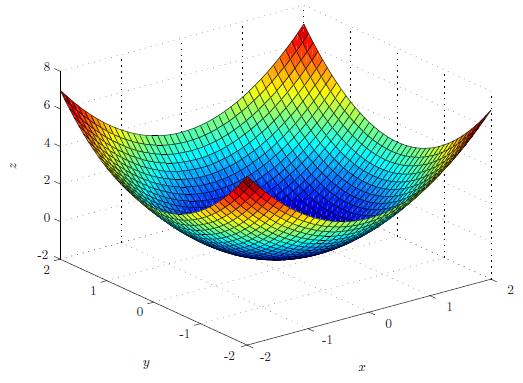
This function looks as follows:

It looks like a parabola in both the -direction and -direction. Now we can calculate the gradient of this function, which is simply:
With this gradient, we have the rate of change in the -direction and -direction in every point where the function is defined. However, now you might wonder: what is the rate of change in some arbitrary direction? We might consider a vector and move along this vector over the graph of the function.
Suppose we are at the point and we want to move along the vector . Being in point , we have a gradient equal to
Meaning that we move +2 in both the -direction and -direction. However, following the path of the vector, we move +2 in the -direction and +1 in the -direction. Hence we move into the -direction and in the -direction, following vector and starting in point . This example is only to illustrate how gradients and vectors work. However, this notion of a directional derivative is important. The formal definition of the directional derivative is the following:
Definition[2]: Directional Derivative in
If , then the directional derivative evaluated at the point is
(If , then the directional derivative evaluated at the point is
Here, denotes the length of the vector. By dividing by , we normalize the vector so that it has unit length.
Using this definition, try to answer the following question.
In the example we previously gave with and , we calculated something that looks like a directional derivative. However, following the definition, can you explain why the one we calculated is not a directional derivative? What does the directional derivative look like in this setting?
This is due to the fact that . Hence we do not have what we call a unit vector. Therefore, we need to normalize this by dividing by the length of the vector. Hence the directional derivative in our case would be:
Hence by following the vector , we move upwards on the graph. Moreover, we use unit vectors because they simplify the proof of the Steepest Descent.
We have something interesting, a directional derivative in a point (which is a vector) and a vector we follow on the graph. We are interested in the direction in which we descend the fastest since we want to arrive at the minimum of the function quickly. If you followed a high school course on mathematics that involved vectors, you are most likely familiar with the following setting and formula:
Angle between two vectors
Suppose we have two vectors and . Then the angle between these two vectors equals:
Or equivalently,
As mentioned before, the directional derivative is a vector, and the vector we follow on the graph is, of course, a vector as well. Let us take and . Then we get:
Where is the angle between the directional derivative and the vector . This angle plays a crucial role in gradient descent. Therefore, try to answer the following question:
For which angle of we descend the fastest and for which angle do we ascend the fastest?
Hint: use the definition of and remember that and is fixed, making
the only variable part.)
Using the hint, the gradient descent method is only influenced by the angle . If we want to descend the fastest, we need to pick the lowest value that the cosine can attain, which equals . This is attained at following the unit circle. This makes sense since the angle of implies that we need to run towards the opposite direction to make a swift descent. This is what is called the Steepest Descent.
Equivalently, we ascend the fastest when the vector and directional derivative point in the same direction. This happens when and thus where . Moreover, this variant is called the Steepest Ascent.
¶ Gradient descent method for optimizing functions
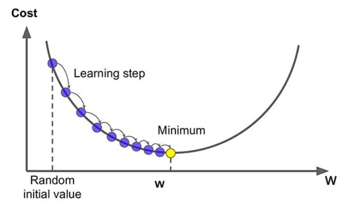
In the last part, you have seen why the method works. In this section, you will see how the algorithm works. As mentioned before, we can use the gradient to approximate the minimum of a function. The gradient of a function at a certain point gives us the graph's direction in that point. Gradient descent is an algorithm that gets us closer and closer to the minimum of a function, using Steepest Descent. It works in steps, so we start at a random initial point, and in each step, we 'walk' in the direction of the minimum such that we get closer after every step. This direction follows from the Steepest Descent, minus the gradient. The picture below illustrates this.

The iteration formula for gradient descent for a function is as follows: where is the current point, is the new point toward which we want to 'walk', is the step size and is the gradient of in the point .
The step size can be chosen; a smaller step size usually leads to more iteration steps but gives a more accurate result. A more significant step size leads to fewer iteration steps but offers a less precise result.
¶ An example
We will do three iteration steps of gradient descent to approximate the minimum of the function .
We start at and use step size .
so .
We can compute the next point: .
For the next step, we first compute .
So .
.
So .
You can see that after each iteration step, we get closer to the point where the minimum is attained, namely x=1 (we have computed this in the first question of this tutorial).
¶ Why use gradient descent?
Using gradient descent in the previous example probably seems way too complicated to compute something simple. Well, this is entirely true. For a function as simple as the one in the example, it is better to find the minimum by setting the derivative to 0. However, as mentioned before, gradient descent gets useful when we have more complicated functions, for example, when we have a function with two variables (a vector function).
Try to do three iterations of gradient descent on the function with starting point
and step size
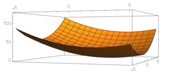
The picture below shows the plot of the function.

and so
We can compute the next point
by
So
We can compute the next point by
So
We can compute the next point by
So
If you look at the plot of the function, you can see that after each iteration step, we get closer to the minimum of the function.
¶ Gradient descent in neural networks
Now that you know the basic idea of gradient descent, you might want to know how we can use this to optimize the flappy bird. To optimize the bird, we want to find the weights for which the bird will perform as best as possible. We will not implement gradient descent in Flappy bird in these tutorials, but we encourage you to try this yourself! To help you a little on your way, we will introduce the notion of a difference function. Suppose that we knew the weights corresponding to the ‘perfect bird’. Then, to get closer to this perfect bird, we need to minimize the difference between our current value and the ideal value. The method of gradient descent can be used to approximate the weights for which the difference between our current bird and the perfect bird is minimal. Try to implement this in your code to get a more advanced AI in Flappy Bird!
¶ Summary
In this tutorial you have learned how to compute the gradient of multivariable functions and how to use gradient descent for optimization. Furthermore, you have seen why gradient descent is a good method to minimize a function. This was the last theoretical tutorial of this track. The next tutorial will give an overview of what you have learned during the whole Flappy Bird track.
Of course, we can use an equivalent variant called gradient ascent for finding the maximum of the function. However, in our case, we want to minimize the errors we make, and therefore we will only consider finding the minimum of a function. ↩︎
This definition can be generalized to multivariable vectors. However, we choose to look at since this is less complicated. ↩︎