¶ Maze lesson 2: extract maze
In case you have any remarks or questions on these tutorials they are always welcome, preferably via the slack channel wiki-content-feedback. (You can notify the education committee specifically by adding @educo to your message.) You may also send us an email at education@serpentineai.nl.
¶ Intro
In this lesson we are going to talk about the following things:
- How to extract the maze from the image.
- How to create a binary image from the maze.
- How to remove sprites.
¶ Binary extraction
The full input image is an RGB image of 512x512. This is a very large image, but it is clear to see that the maze itself can be represented with a much smaller matrix. For this we are going to create a downsampled image of the maze. Downsampling can be done by reducing the width and height of an image, but also by reducing the number of channels an image has. In this case the image has 3 channels because it is an RGB image, but we only really need 1 channel. An image with one channel can be referred to as a gray scale image, or if there are only 2 values, a binary image.
The maze environment normally has a random colored background (left), but to make it ourselves a bit easier this was removed(right):
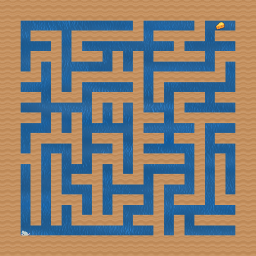
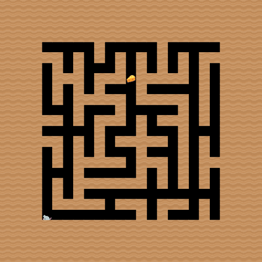
The background was removed by adding use_backgrounds=False to the following line in main.py:
venv = procgen.ProcgenEnv(num_envs=1, env_name='maze', render_mode='rgb_array', use_backgrounds=False)
In the following tabs we will explore how we can simplify the image and get a simple maze image.
- From RGB to Grayscale: learn how to reduce the channels of an RGB image to gray scale.
- From Grayscale to Binary: learn how to reduce the number of colors to 2 values.
- Downsampling: reduce the image size from 512x512 to a much smaller image.
A problem with using the maze as is, is that it contains multiple colors. These colors can make it harder for your algorithm to distinguish between the actual path and walls. To solve this, you can make a function that recolors the maze background. Recoloring is usually done from rgb to grayscale.
Hint: look at OpenCV Module for inspiration
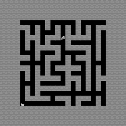
Unfortunately, grayscale is still not clear enough for the algorithm, as there are gradations in gray color. So we have to find a way to make it even easier extract the maze.
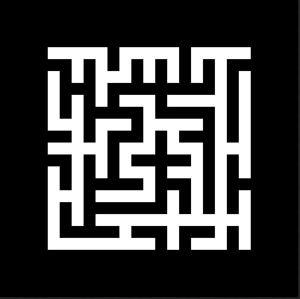
In this tutorial, we go a step further, and convert the found grayscale image to a black and white image (binary colored). By using the output of previous sections we can write a simple function to extract the binary image of the maze.
Hint: take a look at numpy or OpenCV methods for thresholding a grayscale image.
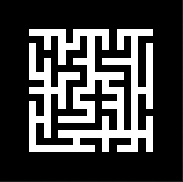
However, as you can see in the resulting image below, the mouse and the cheese are still visable in the binary maze image. This is a problem, since the algorithm will identify the mouse and the cheese as obstacles in the maze, rather than the player and the goal. To remove them, we will have to find their sprite locations in the maze. We will go more in depth into this in lesson 3.
![]()
Side note: officially binary colors are 0 and 1 (black and white), but because the image will be displayed as a gray scale image, the values 0 and 1 both are rendered as black. This makes it very hard to visually see what happens, therefore the values are 0 and 255 instead, which are black and white in gray values.
To process things more easily in later tutorials we want to resize the binary maze. There are 25 blocks in the width and height of the image, each of these tiles either represent a wall (black) or a passable path (white). This number 25 is specific for Maze, and is obtained from the offical environment documentation. The goal is to resize the original 512 by 512 image to a 25 by 25 image.
Hint: OpenCV has a method for this
Code
maze = cv2.resize(maze, (25,25), interpolation=cv2.INTER_LINEAR_EXACT)
There are many other interpolation functions that will work, but we picked INTER_LINEAR_EXACT. From the other options only INTER_NEAREST would not always work correctly.
Other valid options: INTER_LINEAR_EXACT, INTER_LINEAR, INTER_CUBIC, INTER_NEAREST_EXACT, INTER_LANCZOS4 etc...
By downsampling the binary image you can already see that one sprite is removed, the mouse sprite in the bottom left, which is changed to a passable tile (white). The cheese sprite however, is still in there as a wall (black), so we have to find a method to remove this wall since it is actually a passable path, namely the goal.
In order to determine the sprite location on the downsample image we will need the downsample factor. The final method will have to return the donwsampled maze (left image) and the downsample factor, old size divided by new size.
This code should be added to the Agent Class
def extract_maze(self, observation: np.ndarray, grid_size: Tuple[int, int]) -> Tuple[np.ndarray, float]:
    """ Extract the maze from an observation, and downsample it based on the grid size.  """
    gray = cv2.cvtColor(observation, cv2.COLOR_RGB2GRAY)
    maze = np.where(gray, 0, 255).astype(np.uint8)
    maze = cv2.resize(maze, grid_size, interpolation=cv2.INTER_LINEAR_EXACT)
    scaling = tuple(x / y for x, y in zip(observation.shape, maze.shape))
    return maze, scaling[0]
Note 1: this method also returns the ratio between the maze size and the downsampled maze which is something we will use in later tutorials. You can also precalculate this ratio, since it will always be the same.
Note 2: The type hinting for the grid size grid_size: Tuple[int, int], requires the import from typing import Tuple.
¶ Visualization
As you probably have noticed, we are showing a lot of images. This is meant to help visualize what we are doing. It is often very handy to see what your code is producing, because this can help catch early bugs using visual inspection. For this reason we are using the following method inside the Agent class.
    def show(self, image: np.ndarray, window_name: str = '', delay: int = 1, destroy: int = False):
        """ Quickly display an image in this class for testing purposes.  """
        cv2.imshow(window_name, image)
        cv2.waitKey(delay)
        if destroy:
            cv2.destroyWindow(window_name)
This makes it possible to quickly display the maze result using
def compute_action(self, observation: np.ndarray) -> np.ndarray:
    """ Calculate the best action for the agent.  """
    maze, scale = self.extract_maze(observation, grid_size=(25, 25))
    self.show(maze)
    return np.random.randint(0, self.action_space, 1)
Which has helped us to show you the expected results for each of the added stages.
¶ Removing sprites
In lesson 3, we will find the sprite locations of the mouse and the cheese. However, imagine you already have their location, what should you do then? A viable way of removing them from the image is to make them a part of the maze background. Since both are always on a pathway, the pixels of their locations can be converted to the colour of the pathway. In the example below, the pixels of the mouse and cheese locations are converted to a value of 255.
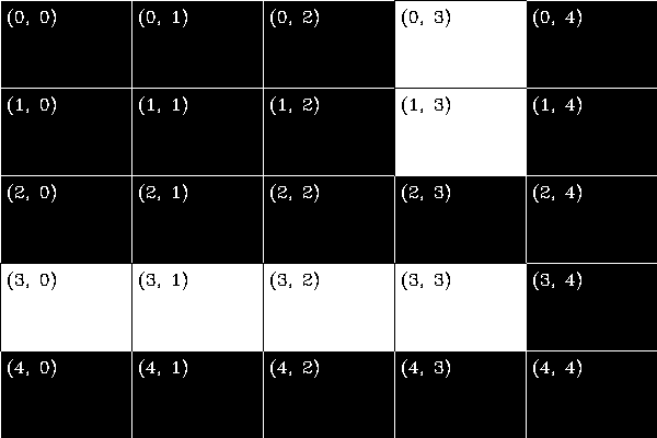
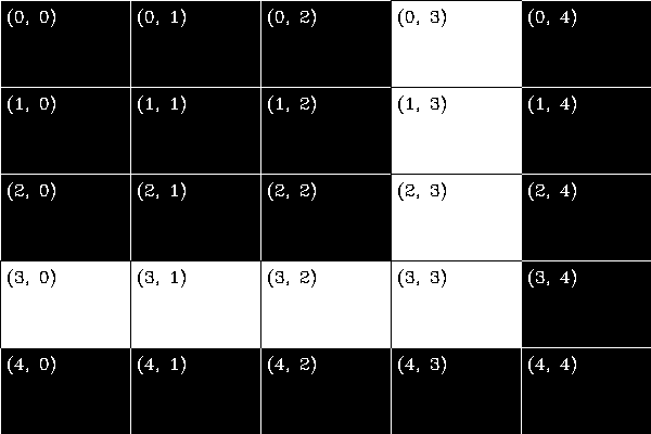
A simple example: Our maze is a 5 x 5 matrix, see left Figure below. In this maze, the white pathway is blocked by a 'sprite' on (2, 3). To remove this blackage we simply have to convert the element of this matrix to white (255). Numpy / cv2 work with (row, col) coordinates, instead of (x, y) and counting starts at 0. Hence the value (2, 3) represents the 3th row and the 4th column value.
maze_bin[2, 3] = 255
Our maze image still has blackage from some of the sprites. So for the next part we ask you to write a general method for removing these sprites form the downsampled maze image.
Hint 1: more examples about numpy slicing.
Hint 2: if you want flexible code, look at bounding boxes (bbox), and how they are defined.
This code should be added to added to the Agent Class
    def remove_sprite(self, image: np.ndarray, sprite_bbox: Tuple[int, int, int, int]) -> np.ndarray:
        """ Removes a sprite from the image (in-place) using their bounding box.  """
        col_min, row_min, width, height = sprite_bbox
        image[row_min: row_min + height, col_min: col_min + width] = 255
        return image
In the downsampled binary image, we can assume that the sprites have width and height of one as well. However to make our method a bit more flexible, it asks for an image and sprite_bbox (sprite bounding box).With the sprite bounding box being a tuple of (left_top_x, left_top_y, width, height).
¶ Summary
In this lesson we have learned how we could simplify the input observation image. This simplification was done by changing the RGB image to a gray scale image and then the gray scale image to a binary image. After this we have downsampled the image to a 25x25 image, and learned how we can remove walls that are actually passable sprites.
In the next lesson we will take a look at how we can locate the sprites.